Enhancements and Modifications to the Full Equations Utilities (FEQUTL) Model, March 1995 to August 1999.
Note: This document is separate from the U.S. Geological Survey report by Franz and Melching (1997). This description of enhancements and modifications to the Full Equations Utilities Model has not been approved by the Director of the U.S. Geological Survey. New subsection for section 1.2, Look-Up Tables, Franz and Melching (1997b), p. 4

Section 1.2.3a Table Interpolation and Automatic Breakpoint Procedure

To RELEASE.TXT

Table Interpolation Procedure and Automatic Breakpoint Assignment

Some general definitions are needed before we can continue with discussion of lookup tables. The points of tabulation of argument used in the lookup tables, to be called function tables from here on, are called breakpoints. These locations are called breakpoints because a discontinuity, a break if you like, in one or more of the derivatives of the approximation, exists there. As an example, consider linear interpolation in a table of values, sometimes called broken-line interpolation. Between the tabulated values the approximation is linear. A linear function is continuous in value and also continuous in its first derivative. However, at each breakpoint, not on the ends of the table, there will be two values of first derivative: one from the line segment on each side of the breakpoint. In general FEQUTL and FEQ will use a polynomial of low degree between tabulated points, that is, linear, quadratic, or cubic, for its interpolation rules. However, at the breakpoints, the level of continuity of the approximation will be lower than the level of continuity between the breakpoints. If the continuity at the breakpoints is only one less than between breakpoints, the interpolating function is called a spline. There are linear splines, quadratic splines, and cubic splines, quartic splines, quintic splines, and so on. These functions are piecewise polynomial functions and they prove to have desirable properties when used to approximate other functions.
FEQUTL uses two methods for the assignment of breakpoints. The first and most frequent is the manual method, that is the user must assign these points in advance of the table computation. This has the advantage of complete flexibility but does require that the user have some knowledge of how the function being tabulated varies. This knowledge varies with the source of the information for the functions and with the experience possessed by the user and the diligence exercised by the user. The second method is automatic assignment of the breakpoints in the table. In this approach the user supplies some general values, such as the minimum value of the argument that is significant, the maximum value of the argument required, and an accuracy goal that the automatic assignment process will hopefully meet.

Benefits of Automatic Breakpoint Assignment

Defining good approximations using piecewise polynomial functions depends on the ability to define good breakpoint locations. Defining good breakpoint locations is not always easy and may require considerable computational effort as well as some degree of cunning in designing the software to accomplish it. Thus we take up some reasons for investing this effort for function tables to be used in FEQ and FEQUTL.
First, the use of the approximation needs to be considered. In the current case, the function tables will probably be accessed many thousands of times in the course of a project. A recent model of about 600 miles of the Mississippi River and its major tributaries upstream and downstream of St. Louis can serve as an example. This model was run for a 25-year continuous period using a three-hour time step. This gives about 73,000 time steps. Let us further assume that there was an average of about 1.5 iterations per time step. Thus each table in the model was accessed for lookup about 110,000 times in that run alone. Many subsequent runs involving periods of several months were done. As another example, models for streams in Du Page County, Illinois, are often run for a series of major runoff events with a total time span of about 2.5 years. The maximum time step is usually 15 minutes but the nature of the stream systems and the storms generally causes the average time step to be ten minutes or less. If we assume about 1.5 iterations for a ten minute average time step we get almost 200,000 accesses to each table in the model. Over a period of several years, this time span may be run many times with many of the tables remaining unchanged. Thus there is considerable justification for an investment in creating tables that have good approximations.
Second, most of the approximations used in function tables in FEQ and FEQUTL use linear splines. This means that the first derivative of the approximation is potentially discontinuous at each breakpoint. The iterative solution processes in FEQ use the first derivative of each function. It is also true that a rigorous convergence analysis for these iterations assumes that not only the first derivative is continuous but also that the second derivative is continuous! In effect the functions as represented in the lookup tables potentially have corners at each breakpoint. If the change in the first derivative at a breakpoint is small there will probably not be any problems with convergence. However, if the corner is too sharp, the possibility for computational problems increases. If the linear spline is a close approximation to the function everywhere then the change in derivative at the breakpoints will be small at all breakpoints. Manual assignment of breakpoints generally does not yield a good approximation at all locations. Consequently there can be significant changes in the derivative that can lead to computational problems. I have had several instances in which failure of the computations in FEQ could be traced to having a breakpoint spacing that was too large in a 2-D table.
Third, manual assignment of breakpoints is often done without careful thought because it is a time-consuming process. In addition the user may not have good knowledge of the pattern of variation of all the functions being computed in FEQUTL. It is common to copy the sequence of breakpoints from an existing source. This manual assignment leads to larger errors in the representation of the function than expected.
Fourth, experience with automatic assignment to date shows that it can materially decrease the total size of some tables even though the overall accuracy of the table is improved. The net reduction in size appears because manual and certain of the current semi-automatic assignment methods concentrate too many points where they are not needed. There are also some tables that will increase in size because their overall accuracy has been increased. In any case, automatic assignment offers the potential of a more nearly uniform level of approximation in the function tables. This will avoid large errors in part of the range and also the waste of breakpoints in parts of the range that are currently represented with an excessive degree of accuracy.
The potential benefits for automatic assignment of breakpoints are large. Not only will it save time on the part of the user in defining the tables but it also will reduce the potential computational problems in the unsteady flow simulation. There may also be some reduction of table size and there will be an increase in the uniformity of approximation accuracy in the tables.
The selection of the sequence of arguments to place in the table with their associated function values is now taken up more formally as part of a broader subject: approximation of functions. The following sections are more mathematical in nature and may be skipped at first reading. However, you should eventually spend some time with them in order to understand how FEQUTL automates the assignment of arguments in function tables. It will also give you some insight into the subtleties of approximating functions.

Approximation of Functions and Function Tables

A function, in the mathematical sense used here, is, "An association of exactly one object from one set (the range) with each object from another set (the domain).", according to James and James(1968). In this broad sense a telephone directory defines a function. The range is the set of telephone numbers in the book and the domain is the set of names in the book. One can quibble about the complication that the same person sometimes has two numbers-those occurrences violate the definition. As any more than cursory attention to mathematics reveals, the nature of the association between objects can take on a wide range of forms.
In our current case, functions are generally relatively simple because all functions of interest to us can be graphed.  All items mentioned earlier in this chapter as being placed in lookup tables are functions in the sense of the definition. FEQ and FEQUTL require that this definition be utilized so that lookup is simplified. In our case the argument for the lookup defines the range of the function. Thus for any value in the range there will be a single value of the function.

Approximation Theory

I have found it useful and convenient to make use of approximation theory, a well developed subject area of mathematics, in constructing function tables. Approximation theory is concerned with using one function to approximate another, usually to save effort in using the function. This has become especially important with digital computers and electronic calculators because these devices only do arithmetic. We have functions, such as the top width, area, conveyance and related functions for a cross section that we have to represent so that the computer can quickly and accurately find a value for any depth in its valid range. The same can be said for the storage capacity of a reservoir, flow through culverts, and so forth. Let  denote the function we want to approximate, sometimes called the approximand, and let  denote the function we will use as our approximant. We will assume throughout that  is continuous and that it has as many continuous derivatives as we need in order for anything we do to make sense. When we are computing an approximation it is only valid over some interval, often only part of the full range of the function. The lower limit of this range will be denoted by  and the upper limit by  in most cases.
We only introduce concepts that are needed and supply only a brief introduction to the methods used in practical approximation. For more details on approximation theory and topics related to it consult one or more of the following sources: Conte and de Boor(1980), de Boor(1978), Dahlquist and Björck(1974). You may also find it useful to refer to calculus texts because these references assume familiarity with calculus and more.

Measures of Closeness

We want the difference between  and  to be small, that is, we want the two functions to be close to each other. The two most useful measures of difference are the absolute difference,  and the relative difference,

where we assume that  to avoid division by zero. Note that these measures only apply at a single point. We also need some way of looking at the collection of differences and deciding if in some sense they are all small enough. We need some criterion for distance between functions, a generalization of the distance between points. When the distance as we define it is small enough we can then say that the function and its approximation are close to each other.
It should be no surprise that there is more than one useful measure of what we mean by the distance between functions. Three useful definitions of distance are:

1. Make the maximum error in absolute value as small as possible. That is

This is also called the Chebyshev error criterion named after a well known Russian mathematician and engineer of the 19th century. His name has been transliterated from the Russian in various ways: Tchebycheff, Tchebychev, or even Cebysev. He developed and applied the criterion in the design of mechanisms made to follow a certain trajectory. If the mechanism deviated too far from its desired path, it could destroy itself as it parts interfered with each other during the motion. Thus this criterion demands that the error be small in some sense at all points in the interval. Creating approximations that best meet the Chebyshev criterion can require extensive computation.

2. Make the integral of the absolute value of the error as small as possible:

This criterion, in distinction from the Chebyshev criterion, only requires that the error be small in an average sense. Obviously, the machinery that Chebyshev was designing would have failed miserably had he only required that the average error be small. The nature of the integral is such that the error can be large over a small interval and still have the criterion be small. This criterion is not often used. However, in some cases it is easy to find approximations with it.

3. Make the integral of the squared error as small as possible, that is, a least squares criterion,

Strictly speaking the distance is given by the square root of the integral. However, if the square is small the square root is small and that is enough for our current purpose. Again this criterion makes the error small in an average sense. One characteristic of least squares approximations is that the error tends to be larger near the ends of the intervals. Approximations using this criterion have a well developed theory and are much easier to compute than those using the Chebyshev criterion. As we will show below, this criterion, modified to use a weight function, can be used to create approximations that come close to satisfying the Chebyshev criterion.
The error used in these definitions of closeness can be either the absolute error or the relative error. We have shown a single example for each criterion for closeness. As should be apparent there are many other possible criteria of closeness between functions but these three are most often used with the Chebyshev and least squares criteria being used most frequently. In all the above definitions we assume that the approximation has one or more parameters that we can vary in order to improve its mimicry of the function. Approximations that satisfy any one of the above criteria are often called best, where best is defined by the criteria. Clearly the approximation will depend on the criterion used in its definition. Furthermore, the criteria we use will depend on the application of the result.
We do not always make explicit use of any of these criteria because the difference between the best approximation and a good approximation is often small, but the effort to develop and establish that an approximation is best can be large. Another good source of approximations is to interpolate values of the function using some rule of interpolation. Once the rule is selected, we can compute some of the errors in interpolation, and check if they are small enough. Clearly if we have good rules for selecting the interpolation points, interpolation will give good approximations of the function.

Selection of Approximating Functions

The motive for using an approximation is that the approximating function, called an approximant, is simpler to compute than the approximand. We select functions that are easy to manipulate and polynomials are the preeminent functions of this sort. They can be evaluated using basic arithmetic; they can also be integrated and differentiated easily. Consequently the bulk of approximation theory centers on polynomial approximation. We have at least two choices here also. The first and classical choice is to use a single polynomial, sometimes of high degree, to approximate the function. As an example, we might try to approximate the logarithm function from 1 to 10 using a single polynomial of some degree. If that is not accurate enough we might try increasing the degree of the polynomial. If we define the polynomial by interpolation and the interpolation points are equally spaced it turns out that there are quite simple functions for which this process does not converge. That is, instead of the error growing smaller as the degree of the polynomial increases, it grows larger. Picking the interpolation points non-uniformly can avoid this problem. (See references above for more detail.)
Using a single high degree polynomial creates an approximant that is global, that is that applies to the entire interval. This may be somewhat simpler in computation but it comes with a price. That is, a change in one point in the approximation, either from roundoff or design, affects the goodness of the approximation at all points, even those that are distant from the point of change. This means that we will experience difficulty in reducing the error locally because an improvement at one location may lead to the opposite effect at other locations. To minimize this behavior, we can use piecewise polynomials as the approximant. That is we select a series of points, called breakpoints within the interval of approximation. Then we use a simple low degree approximation on each of the subintervals. We impose certain continuity constraints at the breakpoints so that the polynomials in adjacent subintervals, called panels, agree in value and perhaps one or more derivatives at their shared breakpoint. To make this concrete, linear interpolation in a table of logarithms is an example of a piecewise approximation. The error is zero at each value in the table and we assume linear variation within each panel. We require that the function value be continuous at each breakpoint but the derivative of the approximation is discontinuous at each break point. This piecewise continuous linear function is called a linear spline. A spline function is a piecewise polynomial function that has one less continuous value at its break points than it does within each of its panels. A linear spline is only continuous in its function value at each break point. However, between breakpoints, it has both a continuous function value and a continuous derivative. If we integrate a linear spline, we get a quadratic spline which has continuous function and derivative values at each breakpoint but has three continuous values in the panels: function, first derivative, and second derivative. Finally if we integrate a quadratic spline we get a cubic spline having continuity of function, first derivative, and second derivative at the breakpoints. That pattern can continue to higher and higher continuity at the break points.
Piecewise polynomials, such as spline functions, are more flexible in following the variations of a function and are also more local in their approximation. For example a change in the value of a linear spline at one breakpoint affects only the adjacent panels. The approximation in other panels is unchanged. Thus when we refine the approximation by adding breakpoints, the other parts of the approximation are unaffected. The quadratic spline is not as local as the linear spline and the cubic spline is less local than the quadratic spline. In either case a change at a breakpoint has a significant effect more or less local to the change with the effect attenuating at more distant panels. In contrast a global approximation will have a significant effect propagate to all parts of the approximation interval essentially unattenuated. The primary spline functions in use in approximation are the linear and cubic splines. Another piecewise cubic polynomial approximation that is useful is a piecewise cubic Hermite polynomial. In this piecewise function each panel is a cubic polynomial but we only require continuity of function and derivative at the breakpoints. We get a higher degree of approximation in each panel but its locality is the same as a linear spline.

Automatic Assignment of Breakpoints

Linear interpolation is used in many function tables in FEQ and FEQUTL. Therefore we will first develop automatic breakpoint assignment for that case. Assignment for higher order interpolation will be developed later.
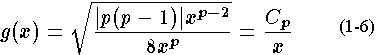
The goal of automatic assignment of breakpoints is to make the errors in linear interpolation small in some sense. Consequently a starting point is to look at an estimate of the error in linear interpolation. A bound for this error in an interpolation interval (a panel) of width,  is given by

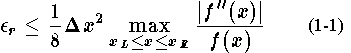
This is the relative error and we always assume that . Notice that the interpolation error can be made small by making the interval of interpolation small. Furthermore, it can be shown that if the breakpoints are selected properly, that this process will converge for a wide class of functions and the rate of convergence will be optimal. See de Boor (1978, pp. 44-47) for more details. The developments below are based on results presented by de Boor. However, he dealt with absolute error and we have generalized the method for relative error.
What we want is some way to measure, on a local basis, the size of the error in linear interpolation for a function that has a continuous second derivative. Equation 1-1 shows that we should use closely spaced breakpoints where the error is large and more widely spaced breakpoints where the error is small. It would be convenient to have some measure of the error per unit length of the argument, a linear-interpolation error density for the function. If we take the square root of both sides of Eq. 1-1 and divide by  we can define a function,  by

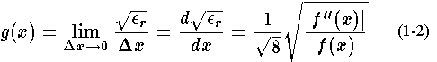
that gives us the derivative of the square root of the relative error of linear interpolation. In other words we have a density, in this case per unit length of argument, of the square root of interpolation error. Knowing this density function we can define a sequence of breakpoints that will be good for interpolation of the approximand, that is, , using a linear spline.
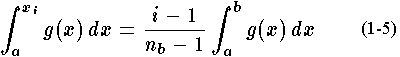
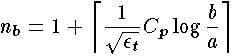
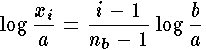
Let the breakpoints of the linear spline be denoted by  where the number of breakpoints, , and . Also denote the target value of the maximum relative error of interpolation by . Now the integral of the density function over an interval gives the square root of the maximum error in linear interpolation over that interval, at least approximately. It will only do this exactly in the limit as the target error approaches zero. However, we are interested in small errors so this looks promising. This means that we want the integral of  over each panel of the linear spline to be . That is

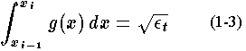
for . Now from Eq. 1-3 we see that we want to find  such that  closely matches . The number of breakpoints must be an integer so we can only do this approximately. So we define  by

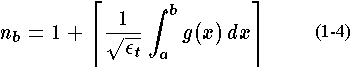
where  denotes the ceiling of its argument, the nearest larger integer number, that is rounding upward to the nearest integer. Once we have defined the number of breakpoints, we then define the interior breakpoints by

for, assigning an equal amount of the error to each panel. This sequence of breakpoints is a good sequence to use in interpolation.
To make this somewhat more concrete, we will work through an example, albeit simple, but yet germane to representing functions needed in unsteady flow modeling. We note that many functions we encounter are close to simple power functions. As examples: flow over a horizontal weir varies as the 1.5 power of the head, flow over a V-notch weir varies as the 2.5 power of the head, flow through an orifice varies as the 0.5 power of the head, the storage in a reservoir often varies at close to the 3.0 power of the depth, and so forth. In reality many of these functions deviate from this variation to some degree. Also some functions will start out with one variation and continue with another. For example, part-full flows in a box culvert with no tailwater influence, will vary approximately as the 1.5 power of the head on the entrance invert. However as the flow becomes larger and the culvert flows full, the flow will transition to variation close to the 0.5 power of the head. In any case let  where  is the power in the simple power function. We can treat the coefficient of the simple power function as 1.0 because we are using relative error. We then find that  and . The density function for the square root of the relative interpolation error becomes

with  is a constant that depends on the power being used. Equation 1-4 gives the number of breakpoints as

and Eq. 1-5 becomes

This last equation becomes

with a slight rearrangement of terms.
Figures 1-1 and 1-2 shows the relative error results when  and  and the target relative error, . Figure 1-1 was computed when , as for flow through an orifice. For simple power functions the linear spline breakpoints assigned by this approach are patterned with a constant ratio. The value of this ratio depends on the power and the target relative error. Figure 1-2 shows the results for  as for flow over a V-notch weir. Note that many more breakpoints are needed in this case even though the range of approximation is the same. The square-root function is closer to linear than a power function with an exponent of . Notice that the errors in each of these two examples varies from zero at the breakpoints to a absolute value that is close to the target relative error. Also note that the linear spline is always on or below the square-root function but that it is always on or above the function, . This follows because the second derivative is of constant sign for each of the two approximands but the sign differs between them. This also means that the error is of constant sign and the approximation will give a consistent underestimate or a consistent overestimate.

The simple functions used in these examples hide some details of implementation. Some of these are:

1. In FEQUTL we cannot in general compute the integrals in closed form because the variation of the function are not simple power functions. Furthermore, it can be relatively expensive to compute hundreds of function values.

2. The functions are only known by numerical computations and so we must estimate the second derivatives numerically. This is done using cubic spline fits to a dense set of points (point set) that we compute. However, the second derivatives are subject to noise from convergence tolerances, coefficient tables, and related sources.

FEQUTL uses the following steps in the computations to select good breakpoint locations:

1. Compute the function values at a fairly dense point set, 30 to 60 points or more, defined assuming the function is a simple power function. That is, the ratio between consecutive argument values in this point set is defined using the approximate power that the function follows. If the power is unknown in detail, the most demanding power is used to make sure that the point set is dense relative to the function.

2. Fit a cubic spline to this dense point set. This cubic spline becomes the surrogate for the real function. Its errors are much smaller than any reasonable target error because the point set is defined for linear interpolation not for cubic interpolation but a cubic spline is used for interpolation.

3. Go through the steps above to define the sequence of breakpoints.

4. Compute the function values at the new breakpoint sequence. Also compute the function value at the midpoint of each panel and use it to estimate the error of linear interpolation.

5. Output the estimated maximum relative error in linear interpolation in each panel.

6. Give summaries of the relative error for the function as a whole and also give root-mean-square error for the function as a whole, estimating the total squared error using Simpson's rule for numerical integration in each panel.

The option for automatic breakpoint selection is available for the commands EMBANKQ and CHANRAT in version 4.52 and later.