 ,
,
Full Equations (FEQ) Model for the Solution of the Full, Dynamic Equations
of Motion for One-Dimensional Unsteady Flow in Open Channels and Through
Control Structures
The equations of motion have as many as three weight coefficients that must be specified. The first weight, present in all four of the governing equation options, is WT, the weight for integration with respect to time. The user has direct control over WT with the FEQ input parameters of BWT and DWT. The value of WT must satisfy 0.5 WT 1 for stability in model simulation. For a linearized form of the equations of motion, WT=0.5 results in the exact numerical result; however, the nonlinear terms in streamflow conditions necessitate the use of a higher value of WT (Lai, 1986). These nonlinear terms affect the solution most if friction losses are relatively small. If the friction losses are small enough, then persistent, nonphysical oscillations in the solution will appear because the solution process, with convective terms, tends to move truncation and roundoff errors to the shorter wavelengths in the solution. In a stream, the energy contained in these shorter wavelengths would be dissipated by processes that take place at a level of detail far smaller than can be resolved with the shallow-water-wave approximations. Furthermore, there is a minimum wave length that can be resolved with the numerical solution. Therefore, the solution contains oscillations at the minimum wave length that cannot be resolved. These oscillations often persist but do not become large enough to result in computational failure as those arising from instability will. By increasing the value of WT, a small amount of dissipation is introduced into the numerical solution. A number of researchers have studied the optimum value for WT. From the standpoint of combining accuracy and stability, Fread (1974) found WT = 0.55 to be the best value for slowly varied unsteady flow such as flood waves, Chaudhry and Contractor (1973) recommended the use of WT = 0.6, and Schaffranek and others (1981) recommended the use of a WT value between 0.6 and 1. In general, values of 0.67 or less are often sufficient to eliminate the oscillations without seriously affecting the accuracy of the final results. The additional dissipation introduced is generally much smaller than the dissipation from boundary friction. In some cases, boundary friction is large enough so that a value of WT = 0.5 can be applied.
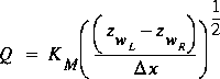
The second weight, WX, also is present in all of the governing-equation options. It is a weight that is computed internally to adjust the computation of friction losses at small depths to avoid convergence problems in the numerical solution of the system of nonlinear equations. Following the work of Cunge and others (1980, p. 175-178), the value of this weight is computed to obtain a single-valued solution at shallow depths. To illustrate this approach, a simple approximation to the motion equation when all inertial terms are suppressed is considered, resulting in
(81)
,
where KM is a mean value of conveyance in the control volume,  is the water-surface elevation at the left (upstream) end of the control volume, and
  is the water-surface elevation at the right end of the control volume. If the elevation on the left is held constant and the elevation on the right is allowed to decrease, the flow will increase for a time because the increase in slope more than compensates for the decrease in the conveyance. However, when the elevation on the right decreases below some level that depends on the two water-surface heights and the variation of conveyance, the flow will no longer increase. Thus, for a given flow, two values of water-surface height could satisfy the equation. Thus, the numerical solution may not converge because of this duplication of solutions at shallow depths. This convergence problem can be solved by changing the definition of KM so that more weight is given to the upstream point and so that the partial derivative of the flow with respect to the right-hand elevation is always negative.
If 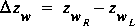 is the change in water-surface elevation, KM = KL + WX(KR - KL) is the average value of the conveyance, and Sw = -
 zw/x is the water-surface slope with a decline in elevation given a positive slope, then
(82)
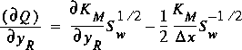 .
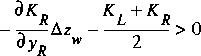
.Multiplying equation 82 by Sw1/2, requiring that the rate of change of flow with change in the right-hand water-surface elevation always be negative, and substituting the value for KM results in
(83)
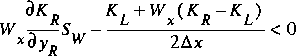 ,
,as the defining inequality. If this inequality is not satisfied when WX = 0.5, then the value of WX must be changed so that the inequality will be satisfied when WX < 0.5. The value of WX that will satisfy the inequality is
(84)
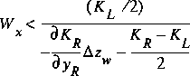 .
.The denominator in this equation is always positive, given that
(85)
 .
.The inertial terms have been ignored in the analysis up to this point. These are usually small when the water-surface height is small enough for this correction to be required. To allow for some consideration of these effects and to prevent the rate of change from becoming zero, a value of 0.8 of the right-hand side of the inequality in equation 84 is applied as the value for WX in the FEQ simulation. The flow of water is assumed to be from left to right in the analysis. Similar relations are used when the flow of water is from right to left.
The third and last weight, WA, is applied only in the options STDW and STDCW. This weight applies to certain integrals with respect to distance to allow computation of unsteady flows at small depths. The preceding small-depth adjustment allows receding flows to be computed to depths that are near zero; however, the computations may fail when the flows begin to increase from small depths unless the rate of increase with time is much smaller than for most stream rises. When the depths are small and an increase in flow begins, the errors of approximation in the distance integrals can become large. If  and
and  in the conservation of mass equation 68 are given the value 0.5, the distance integrals are approximated with the trapezoidal rule, and the integrand is assumed to vary linearly in the integration interval. When the depths are large, a linear approximation to the variation of flow area with distance results in a relatively small error. Equation 68 is exactly applied in the solution process, but this may require that either the left-hand or the right-hand area be negative whenever the flow increases from a small value. A negative area is impossible, so the computations fail. However, if the value of WA is increased, giving more weight to the downstream point, equation 68 can be satisfied without resulting in a negative area. The value of WA will approach 1.0 when the depths are very small. High values of WA have larger apparent integration errors than does a value of 0.5, but in most applications, the details of the flow at small depths are not of great interest. Thus, some increase in error at these depths is acceptable in order to allow the computations to continue. If the small depths are of interest, then the user must reduce the length of the computational elements so that the small depths can be simulated without applying a variable WA.
The values for WA are defined by the user for each branch in the system. A typical depth below which the value of WA becomes virtually 1 and a typical depth above which the value of WA becomes 0.5 must be given for each branch. Values of the weight for depths intermediate to these two are determined by either linear or cubic interpolation, at the user's request.