Full Equations (FEQ) Model for the Solution of the Full, Dynamic Equations of Motion for One-Dimensional Unsteady Flow in Open Channels and Through
Control Structures
In general, even a single nonlinear equation cannot be solved without some numerical method to approximate the solution to the equation. The example of a single equation illustrates some of the problems that are considered in FEQ simulation. Thus, Newton's iteration method for solution of nonlinear equations is initially described and illustrated for the case of a single nonlinear equation. The discussion of Newton's method is then expanded to the simultaneous solution of many equations.
where
![]() is the value on the line tangent to FN
, the point of tangency being
is the value on the line tangent to FN
, the point of tangency being
![]() . Solving equation 124 for u where
. Solving equation 124 for u where
![]() = 0 yields the root for the tangent line,
= 0 yields the root for the tangent line,
(124)
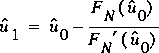 ,
,
where
![]() is the root of the tangent line, which becomes the
next approximation to a root of the equation. This process can
be repeated until the approximations to the root approach some
limit or until the value of the function FN
becomes acceptably small. Equation 124, rewritten to show this
process, becomes
is the root of the tangent line, which becomes the
next approximation to a root of the equation. This process can
be repeated until the approximations to the root approach some
limit or until the value of the function FN
becomes acceptably small. Equation 124, rewritten to show this
process, becomes
(125)
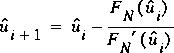 ,
, where i= 0, 1, 2, . . . Various applications of Newton's method are shown in figure 18.
Cases that can result in problems in the convergence of Newton's method are shown in figure 18b-d. In the first case, the root is near a point of inflection so that the iterations oscillate and convergence is impossible. In the second case no root is possible: Newton's method will not converge because there is no root to converge to. In the third, the derivative is zero at a root, so the method may not converge or will converge slowly. Hamming (1973, p. 70-72) and Dennis and Schnabel (1983, p. 21-23) discuss means for detecting these problems for a single equation.
As an example of the application of Newton's method, consider
two equations and two unknowns. To distinguish the iteration
number from the number used to denote the variable, let a
superscript denote the iteration number, and not an exponent.
If there are exponents, they must be set off with parentheses.
For example,
![]() denotes the initial value for the first unknown in the vector
u,
denotes the initial value for the first unknown in the vector
u,
![]() denotes the second iteration as it affects the first unknown,
and
denotes the second iteration as it affects the first unknown,
and
![]() denotes the square of the value of the second unknown at the
second iteration. Discarding all nonlinear terms from a Taylor
series expansion about the point u 0 yields
two equations:
denotes the square of the value of the second unknown at the
second iteration. Discarding all nonlinear terms from a Taylor
series expansion about the point u 0 yields
two equations:
(126)
(127)
Setting each of these equations to zero and solving for the unknowns gives the first-iteration results for the roots of F 1 and F 2 as for a single equation. Two linear equations in two unknowns result. However, the notation becomes unmanageable as the number of equations increases. FEQ simulation can involve several thousand equations and as many unknowns. Matrix notation makes for a more compact and more general display of the equations and the solution process. Equation 123 in matrix notation is
where u is the vector of values on the tangent planes, F(u) is the vector of values of the residual functions for the equations, and J( u) is the matrix of partial derivatives of the residual functions, called the Jacobian matrix. If ne = 2, then
(129)
 ,
, (130)
 ,
, (131)
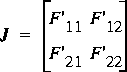 .
. In equation 128, the argument list following a vector or matrix symbol is applied to each element of the vector or matrix.
Letting
![]() and solving for the approximation to the root results in
and solving for the approximation to the root results in
(132)
as the final form of the iteration for a simultaneous system of nonlinear equations by means of Newton's method. In equation 132, J -1 denotes the inverse matrix for the Jacobian of the system of equations. Dennis and Schnabel (1983, p. 21-23) discuss the conditions for convergence of Newton's method for a system of nonlinear equations. The convergence is quadratic if the first derivatives are sufficiently smooth and the initial point is not too far from one of the roots of the equations.
Obviously, the solution of a system of nonlinear equations is much more complex than for a single equation. Similar convergence problems may result, but now no simple geometric visualization is possible. Furthermore, Dennis and Schnabel (1983, p. 9) point out that problems involving 50 or more equations are difficult to solve unless a good estimate is available before iteration. However, this is only true for systems in which the Jacobian matrix is filled, or nearly so, with nonzero elements. In one-dimensional, unsteady-flow analysis, the Jacobian has a special structure and contains many zeros. For large stream systems, less than 1 percent of the elements in the Jacobian will be nonzero; all other elements are known in advance to be zero. This structure is used in FEQ simulation to reduce the complexity and number of computations.